adamdawes.com - Tokamak Physics

Home Programming Tokamak PhysicsTutorial 2, colliding cubes

Tutorial 2, colliding cubes

Now its time to get started with using the Tokamak engine in our project. This tutorial is fairly simple but due to the nature of the physics engine it's great fun to watch. I must have run this program hundreds of times now just to watch it over and over again (perhaps I'm just easily pleased!).

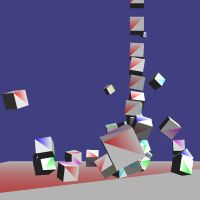
This tutorial will model dropping a number of cubes positioned vertically above one another so that they fall to the floor beneath. When they hit the floor they will begin to stack up on top of one another until after a short while the stack becomes unbalanced, which usually results in it collapsing completely to the floor, sending the cubes flying in all directions. The zip file at the bottom of the tutorial contains an executable for the project (as well as all the source code) if you want to have a look at what it does before getting back to how it does it.

Before we get carried away we need to do a little preparation: we need to configure the C++ compiler so that it is able to use the Tokamak engine, and we need to understand a little of what we're going to be doing.

Compiler configuration

Before we can write any code that uses the Tokamak engine we need to install the SDK. This can be downloaded from the Tokamak Physics web site. At the time of writing the latest version (against which these tutorials have been compiled) is v1.0.8. The Tokamak team release new versions containing enhancements and bug fixes on a regular basis, but hopefully the later versions will continue to work with these tutorials. Once the SDK is downloaded, extract all of the files to your hard drive (making sure to keep the directory structure that is present within the zip file).

There are two primary components of the SDK that we'll need in order to compile our code. The first is the .lib file that we need to link with. This contains the actual compiled program code that forms the Tokamak engine. Secondly we'll need the include files in order for the compiler to know how to communicate with Tokamak.lib.

So that MSVC knows how to find these files, we need to add the appropriate folders to the IDE. To accomplish this in MSVC6, follow these steps (the procedure may be different for MSVC .net):

Select Tools>Options from the MSVC menu
Click on the Directories tab
Ensure "Include files" is selected in the "Show directories for" list
Double-click the empty box at the bottom of the directory list so that it becomes editable
Click the "..." button and browse to the "include" folder in the location where the SDK was extracted
Click OK to return to the Options window; the path should now be present in the directory list.

Once this is done, change "Show directories for" to show the directories for Library files. Repeat the above steps, browsing to the "lib" folder of the SDK. Once this is finished, click OK on the Options window to return to the main IDE.

The compiler is now configured for using the Tokamak SDK. These steps only need to be performed once and are not required the next time you start up MSVC.

Understanding the physics engine

The Tokamak engine has quite a number of variables and parameters that can affect the way in which it works. For this sample we'll be keeping things as basic as possible but there are some terms that need explaining before we get started.

Tokamak hinges around a class called neSimulator. This class is used to access all of the items of the physics engine and is also responsible for updating the positions of all the objects as the simulation runs.

There are two main types of object used in the simulation: rigid bodies and animated bodies. Rigid bodies are those for which the movement is completely controlled by the simulator; animated bodies are those for which the simulator will never change the position, these bodies are only ever repositioned by the application itself. For our sample, the floor will be an animated body and the cubes we drop towards it will be rigid bodies.

Bring on the code

So, let's get started with the code that will drive the application.

The very first thing we need to do is include the "tokamak.h" header so that the compiler knows about the functions available on tokamak.lib. We also need to instruct the linker to include tokamak.lib when building the final executable. This can be achieved using the Project Settings dialog, but I prefer to use the #pragma compiler directive (it's easier to spot the libraries that are used, and it doesn't get lost when changing between Debug and Release builds).

#include <tokamak.h> #pragma comment(lib, "tokamak.lib")

Next we initialise a few variables for Tokamak itself. These should probably be nicely packaged into a class but for the sake of simplicity they're simply defined as globals in this code.

// Global variables for Tokamak neSimulator *gSim = NULL; // The number of cubes to render in the simulation (try values between 2 and about 50) #define CUBECOUNT 5 neRigidBody *gCubes[CUBECOUNT]; neAnimatedBody *gFloor = NULL;

gSim is the simulator object itself. Then we have an array of rigid bodies, each of which will represent one cube in our simulation, and a single animated body to represent the floor. The only other addition to this section of code is the vertex data for the floor (vbFloor is the vertex buffer, and gFloorVertices holds the floor vertex positions).

The next change is to the WinMain procedure. Along with all the other initialisation and shutdown functions, two new functions are called: InitPhysics is responsible for initialising the simulation and positioning all the objects ready for the application to start, and KillPhysics tidies everything up once we're finished.

Let's take a look now at InitPhysics. After declaring some variables for use within the code we start to prepare for creating the main simulator object.

The first thing the simulator needs when it is created is a neSimulatorSizeInfo object, populated with information about the bodies that are going to be simulated. This needs to be provided up- front so that Tokamak can allocate all the required memory before the simulation begins. This is quite significant as it means you need to know the maximum number of objects you will need to simulate at the point of initialisation.

The relevant information for the moment is the number of rigid and animated bodies, and the maximum number of simultaneous "overlapped pairs" of objects possible within the simulation (an overlapped pair represents the potential collision between any two objects). This isn't quite as nasty as it sounds, and can be calculated using a fairly simple formula as shown below.

The code so far to prepare the neSimulatorSizeInfo object is as follows:

// Initialise the Tokamak physics engine. // Here's where the interesting stuff starts. bool InitPhysics(void) { neGeometry *geom; // A Geometry object which used to define the shape/size of each cube neV3 boxSize1; // A variable to store the length, width and height of the cube neV3 gravity; // A vector to store the direction and intensity of gravity neV3 pos; // The position of a cube f32 mass; // The mass of our cubes neSimulatorSizeInfo sizeInfo; // Stores data about how many objects we are going to model int i; // Create and initialise the simulator // Tell the simulator how many rigid bodies we have sizeInfo.rigidBodiesCount = CUBECOUNT; // Tell the simulator how many animated bodies we have sizeInfo.animatedBodiesCount = 1; // Tell the simulator how many bodies we have in total s32 totalBody = sizeInfo.rigidBodiesCount + sizeInfo.animatedBodiesCount; sizeInfo.geometriesCount = totalBody; // The overlapped pairs count defines how many bodies it is possible to be in collision // at a single time. The SDK states this should be calculated as: // bodies * (bodies-1) / 2 // So we'll take its word for it. :-) sizeInfo.overlappedPairsCount = totalBody * (totalBody - 1) / 2; // We're not using any of these so set them all to zero sizeInfo.rigidParticleCount = 0; sizeInfo.constraintsCount = 0; sizeInfo.terrainNodesStartCount = 0;

The other thing required to initialise the simulator is a vector that represents gravity. Normally gravity is obviously directed straight down (with a negative y value), but you can have gravity set to be in any direction you like -- including upwards if you want. Larger values represent a stronger pull along the appropriate axis. We set the gravity direction as follows:

// Set the gravity. Try changing this to see the effect on the objects gravity.Set(0.0f, -10.0f, 0.0f);

With the size and gravity data all set we can finally create the simulator object.

// Ready to go, create the simulator object gSim = neSimulator::CreateSimulator(sizeInfo, NULL, &gravity);

With the simulator created we are ready to create the objects we wish to simulate. We'll set up a loop for each of our cubes, and get the simulator to create a rigid body for each one. The pointer to the rigid body is placed into the gCubes array.

// Create rigid bodies for the cubes for (i=0; i<CUBECOUNT; i++) { // Create a rigid body gCubes[i] = gSim->CreateRigidBody();

The simulator now knows that we have a rigid body, but it doesn't know anything about its shape or size. Tokamak uses three primitives to represent the shape of an object that it is going to simulate. These are the box, cylinder and sphere. Each time you add a body to the simulation you will need to create the geometry for the body using these primitives. A body may have multiple geometries associated with it if it has a more complex shape, but as we are only modelling cubes in this tutorial we can simply use a single box primitive for our geometry.

In the code below we set the size of the box to (1, 1, 1). These values match with those used in the vertex data for the cube at the top of the source code (the cube extends from -0.5 to +0.5 along each axis, giving a size of 1.0). The three values used below correspond to the X, Y and Z axes respectively; changing the size of the cube in the vertex data will require the values below to be updated accordingly if the simulated object is to match its representation drawn on the screen.

Every time the geometry for a body is set or modified, the UpdateBoundingInfo method of the object must be called. This instructs Tokamak to update its simulation for the geometry data that has been set. If this is not called, your objects will probably fall straight through the floor without ever colliding with it.

// Add geometry to the body and set it to be a box of dimensions 1, 1, 1 geom = gCubes[i]->AddGeometry(); boxSize1.Set(1.0f, 1.0f, 1.0f); geom->SetBoxSize(boxSize1[0], boxSize1[1], boxSize1[2]); // Update the bounding info of the object -- must always call this // after changing a body's geometry. gCubes[i]->UpdateBoundingInfo();

Next we set some other properties of the body: mass and the inertia tensor. The mass of an object represents how "heavy" it is in relation to other objects in the scene. If an object with a small mass collides with an object with a large mass, the large mass object will be relatively less affected. This is not so easy to see in this simulation as all the cubes have the same mass value.

The inertia tensor is similar to mass, but whereas mass relates to the change in position of an object, the inertia tensor relates to the change in rotation of an object. We'll use the helper function neBoxInertiaTensor to set this for us; remember to use the help function that corresponds to the type of geometry that's been used for the body.

// Set other properties of the object (mass, position, etc.) mass = 1.0f; gCubes[i]->SetInertiaTensor(neBoxInertiaTensor(boxSize1[0], boxSize1[1], boxSize1[2], mass)); gCubes[i]->SetMass(mass);

Finally we just need to position the cube in space ready for it to be simulated. For this application, we'll position each cube vertically one above the other with a gap between each. All the cubes will be dropped simultaneously however, so cubes higher up will be travelling faster by the time they reach the ground due to the increased acceleration of gravity acting upon them. We'll also provide a slight randomisation on the X and Z axes so that the stack is more likely to fall over (it makes it much more interesting to watch).

// Vary the position so the cubes don't all exactly stack on top of each other pos.Set((float)(rand()%10) / 100, 4.0f + i*2.0f, (float)(rand()%10) / 100); gCubes[i]->SetPos(pos); }

And that's all our cubes ready to run. If it looked complicated, try changing some of the values around and running the simulation to see what effect the changes have on the cubes.

Next we need to create the animated body that will represent the floor. This is all pretty much identical to how we created the cubes, except the we call CreateAnimatedBody instead of CreateRigidBody. We'll set the floor to have very little height, and to have its width and depth as defined by our FLOORSIZE constant. We'll also set the floor so that it's centered on the X and Z axes, but positioned a little way below the origin on the Y axis.

// Create an animated body for the floor gFloor = gSim->CreateAnimatedBody(); // Add geometry to the floor and set it to be a box with size as defined by the FLOORSIZE constant geom = gFloor->AddGeometry(); boxSize1.Set(FLOORSIZE, 0.2f, FLOORSIZE); geom->SetBoxSize(boxSize1[0],boxSize1[1],boxSize1[2]); gFloor->UpdateBoundingInfo(); // Set the position of the box within the simulator pos.Set(0.0f, -3.0f, 0.0f); gFloor->SetPos(pos); // All done return true; }

That's the end of InitPhysics, from here our similation is ready to run. KillPhysics simply releases the simulator object (if it's been set). This will automatically clear up all bodies, geometry and other objects that have been associated with the simulator so there's no need to tidy up any further than this.

void KillPhysics(void) { if (gSim) { // Destroy the simulator. // Note that this will release all related resources that we've allocated. neSimulator::DestroySimulator(gSim); gSim = NULL; } }

The final addition to the code in unsurprisingly in the Render function. There are two new things we do here: firstly we advance the simulation so that it updates all the positions of the objects, and secondly we draw the objects to the screen.

The simulation is advanced by calling the Advance method of the simulator object. This method expects the amount of time that has passed since the last time we made the call to be passed so that it knows how far to move each object in the simulation.

There are also two optional parameters to Advance: the first, nSteps is the number of sub-divisions of the time frame to be used for object calculations. For example, if 1/60th of a second has passed, we could call with 1/60 as the time parameter, passing 1 for the number of steps. If we passed 2 for steps, it would be equivalent to calling Advance twice with 1/120 as the time parameter and a step of 1. Larger values of step provide a more "accurate" simulation but at the cost of decreased performance. For most purposes a step of 1 is sufficient.

Advance is also able to return a performance report object so that we can query how long it took working on each part of the simulation update. This is not something used in this tutorial, however.

As we can use our timer to determine exactly how much time has passed (in seconds), we'll use this value to ensure that the simulation always runs at the same speed, regardless of frame rate or processing power. However, one slight complication with this method is that the Tokamak engine works best with a fairly constant time interval passed each time it updates. Unexpected variations can cause the stability of the engine to fluctuate, often resulting in extreme movement of the objects being simulated.

To avoid this, we'll try to ensure that the elapsed time never varies by more than 20% of what is was the previous time we called Advance. We will also ensure that no time interval lasts longer than 1/45th of a second, as updates slower than this can also cause problems within the simulation. The following code retrieves the elapsed time and smooths out the values based on these principles. [Thanks to Chris Chan at Tokamak for pointing this issue out to me]

float fElapsed; static float fLastElapsed; [...] // Find out how much time has elapsed since we were last called fElapsed = GetElapsedTime(); // Prevent the elapsed time from being more than 20% greater or // less than the previous elapsed time. if (fLastElapsed != 0) { if (fElapsed > fLastElapsed * 1.2f) fElapsed = fLastElapsed * 1.2f; if (fElapsed < fLastElapsed * 0.8f) fElapsed = fLastElapsed * 0.8f; } // Stop the elapsed time from exceeding 1/45th of a second. if (fElapsed > 1.0f / 45.0f) fElapsed = 1.0f / 45.0f; // Store the elapsed time so that we can use it the next time around fLastElapsed = fElapsed;

Now that we've calculated an acceptable time period for which to advance the simulation, we'll pass it to the simulator's Advance method to update the objects.

gSim->Advance(fElapsed);

With the simulation updated we now need to ask it for the positions of each of our objects so that we can render them. We'll start with rendering the floor. Even though the object won't be moved by the simulation itself (it's an animated body), we'll still query the position from the engine to ensure we are displaying it in the position that the engine believes it to be.

We retrieve the position of the floor by calling the GetTransform method of the floor's body object. This returns a matrix containing all of the positional data we need. However, it's not in quite the same format that DirectX requires in order for it to set the position for rendering, so we need to transfer the values out of the Tokamak matrix object and into a DirectX matrix object. (For an OpenGL application, this transfer would need to be modified in response to the different coordinate system used by OpenGL.)

Once this is done we simply set the world transformation and render the floor.

// Set the vertex stream for the floor gD3DDevice->SetStreamSource(0,vbFloor,sizeof(strVertex)); // Draw the floor... // Get the transformation matrix for the floor object t = gFloor->GetTransform(); // Transfer the values to a D3DMatrix that we can pass to DirectX dxTrans = D3DXMATRIX( t.rot[0][0], t.rot[0][1], t.rot[0][2], 0.0f, t.rot[1][0], t.rot[1][1], t.rot[1][2], 0.0f, t.rot[2][0], t.rot[2][1], t.rot[2][2], 0.0f, t.pos[0],t.pos[1], t.pos[2], 1.0f ); // Set the world transformation so that we can draw the floor at the correct position gD3DDevice->SetTransform(D3DTS_WORLD, &dxTrans ); // Render the floor gD3DDevice->DrawPrimitive(D3DPT_TRIANGLELIST,0,2);

The code to render the cubes is essentially identical, using each cube's body to determine the position for rendering.

// Set the vertex stream for the cube gD3DDevice->SetStreamSource(0,vbCube,sizeof(strVertex)); // Draw the cubes for (i=0; i<CUBECOUNT; i++) { // Get the transformation matrix for this cube t = gCubes[i]->GetTransform(); // Transfer the values to a D3DMATRIX that we can pass to DirectX dxTrans = D3DXMATRIX( t.rot[0][0], t.rot[0][1], t.rot[0][2], 0.0f, t.rot[1][0], t.rot[1][1], t.rot[1][2], 0.0f, t.rot[2][0], t.rot[2][1], t.rot[2][2], 0.0f, t.pos[0],t.pos[1], t.pos[2], 1.0f ); // Set the world transformation so that we can draw the cube at the correct position gD3DDevice->SetTransform(D3DTS_WORLD, &dxTrans ); // Render the cube gD3DDevice->DrawPrimitive(D3DPT_TRIANGLELIST,0,12); }

...And that concludes the code required for this tutorial. I think you'll agree that with very little code an astounding level of realism can be obtained even if we are only looking at cubes on a flat surface. Because of the complexity of the calculations involved and the fact that the timing will not be identical every time the application runs, the simulation is never the same twice. This can make it very interesting to watch but also potentially unpredictable in practise so be careful!

Feel free to experiment with changing the number of cubes simulated, the floor size, gravity, and even the size of the cubes (it's very little work to make them look like dominos).

The source code and a compiled executable for this tutorial are available in the following .zip file.

TokamakTutorial2.zip

<< Tutorial 1, the DirectX framework <<

>> Tutorial 3, cylinders and spheres >>

If you have any comments or suggestions regarding this article, please don't hesitate to contact me.